If you’ve read my earlier post on Conditional Variational AutoEncoders, this should be a piece of cake. If you understand a regular VAE, you're already 90% of the way to understanding a Vector Quantized - VAE. The only thing you need to change in your thinking is what the "latent space" or "bottleneck" looks like.

In a standard Variational AutoEncoder (VAE), the encoder takes an image and maps it to a point on a smooth, continuous "map" (the latent space). You can pick any point in this space, even one between two learned points, and the decoder will generate a corresponding image. This is like a painter who can mix any color on a continuous color wheel.

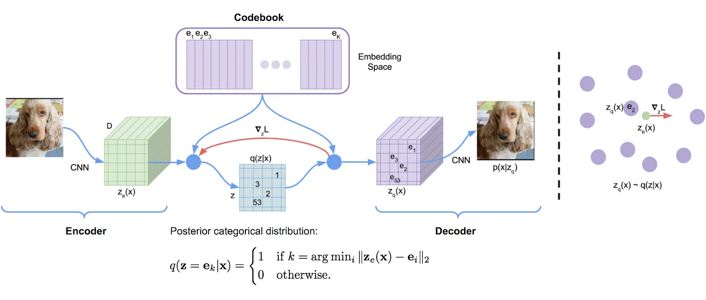
A Vector Quantized-VAE (VQ-VAE) is different. Instead of a continuous smooth map (or a probability distribution), it has a finite codebook (a collection of vectors), which is like a dictionary of "visual words".

The Process:

1. The encoder takes an image and produces a set of vectors, just like a VAE.
2. But then, instead of keeping those vectors, the VQ-VAE looks up the closest matching vector in its codebook and replaces the encoder's output with that vector. It's a "snap-to-grid" step.
3. The decoder then receives this sequence of vectors from the dictionary to reconstruct the image.

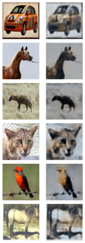
This simple change from a continuous map to a discrete dictionary has one huge benefit: it solves the "blurry image" problem that often affects VAEs. Because the VQ-VAE is forced to choose a specific "word" from its dictionary, it can't hedge its bets by averaging between two possibilities. It has to make a firm decision. This forces the decoder to learn how to reconstruct sharp, high-quality images from a limited but precise set of building blocks.

Recall the loss function for a standard VAE, which is the negative Evidence Lower Bound (- ELBO)

$L_{VAE}=E_{q(z∣x)}[logp(x∣z)]−D_{KL}(q(z∣x)∣∣p(z))$

• Reconstruction Loss: This term trains the decoder to reconstruct the input x from a latent sample z.
• KL Divergence: This is a regularization term that forces the encoder's approximate posterior distribution q(z|x) to be close to a simple prior distribution p(z)

The VQ-VAE uses a deterministic encoder and a discrete codebook (a categorical distribution). The prior distribution is no longer continuous. This means the KL divergence term is no longer applicable. It's replaced by two new loss terms designed to train the codebook.

The overall VQ-VAE loss is:

$L_{VQVAE}=∥x−x∥^2+∥sg[z_e(x)]−e_k∥^2_2+β∥z_e(x)−sg[e_k]∥^2_2$

The 1st term is the simple MSE loss for reconstruction.

The probabilistic encoder q(z|x) is replaced by a deterministic encoder that outputs a vector z_e(x). This vector is then mapped to the nearest codebook vector e_k in a non-differentiable step:

$k=argmin_j∥z_e(x)−e_j∥^2_2$

The 2nd term updates the codebook vectors. The sg[] is the stop-gradient operator, which treats its input as a constant during backpropagation. Here, it blocks the gradient from flowing to the encoder. It pulls the chosen codebook vector e_k closer to the encoder's output z_e(x). This is how the "dictionary" of codes learns to represent the data.

The 3rd term updates the encoder. The stop-gradient now blocks the gradient from flowing to the codebook. It pushes the encoder's output z_e(x) to stay "committed" to the codebook vector e_k it was matched with. This prevents the encoder's outputs from growing uncontrollably or drifting along the codebook vectors.

The architecture of a VQ VAE is simple enough. An encoder that outputs vectors, a vector quantizer that picks the closest vectors from its embeddings, & a decoder that takes in the vectors and outputs an image.

I trained a simple VQ VAE on the CIFAR 10 dataset. A small 6 layer Relu activated encoder with convolution layers followed by residual blocks. Same as the decoder but with transposed convolutions for upsampling. The quantizer with an embedding layer (512x128) and 0.25 as the beta for the commitment loss. This model turned out to have 1.5 million parameters. Great! (or so I thought). I trained it for 10 epochs. It took about 2 hours to train on a T4 GPU. the results are not all that great. I am also trying a Bayesian Hyperparameter Search with different batch sizes, activations and residual blocks. Fingers crossed 🤞.

In the next post we’ll go over Hierarchical VQ VAEs and how to conditionally generate images using learned priors.

Sources -

Original Paper by Oord et al.

https://huggingface.co/blog/ariG23498/understand-vq

https://shashank7-iitd.medium.com/understanding-vector-quantized-variational-autoencoders-vq-vae-323d710a888a